Analysis of sorting algorithms
Sorting algorithms are one of the most basic as well as one of the most used algorithms. They form the basis for many other data structures and algorithms and are also a great way to learn to analyse algorithms.
In this post, I would like to perform my own analysis of these sorting algorithms to understand where and why various sorting algorithms should be used. My main focus is going to be practical analysis of these sorting algorithms and I am also going to be considering the simplicity of these algorithms.
So first, let us think about what basis we are going to use for these sorting algorithms. To analyse any sorting algorithm, let us measure the time it takes to sort an array of integers. The array of integers that we are going to give to the sorting algorithms should be of the following types:
- Random arrays. Ex:
[5, 2, 9, 7, 0, 4]. - Sorted arrays. Ex:
[3, 5, 7, 8, 11]. - Sorted arrays in reverse order. Ex:
[14, 11, 7, 3, 1]. - Sorted arrays with a few random elements added to the end. Ex:
[1, 4, 5, 9, 11, 19, 2, 18, 5]. - Sorted arrays with some random elements mixed in between. Ex:
[1, 3, 37, 5, 6, 11, 9, 14, 2, 25]. - The above types but with a lot of duplicate elements.
Random arrays can easily be generated by just adding random numbers to the array.
Sorted arrays can be generated by adding a random number to the previous element.
Reverse sorted arrays can be generated in a similar manner as the sorted arrays.
The rest of the types of arrays are just a mixture of the techniques used to generate random, sorted and unsorted arrays.
If you would like to like to check my version of the analyser, you can head over to this Github repository.
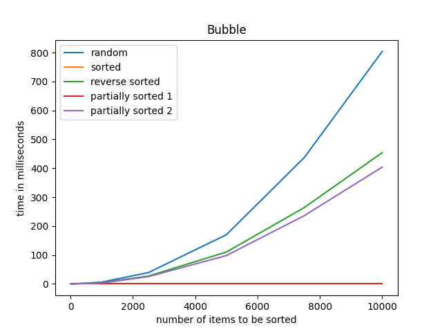
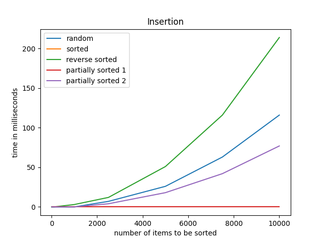
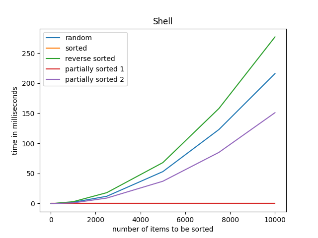
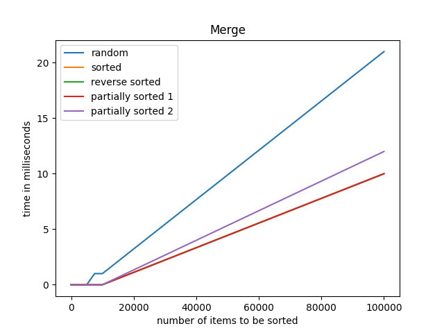
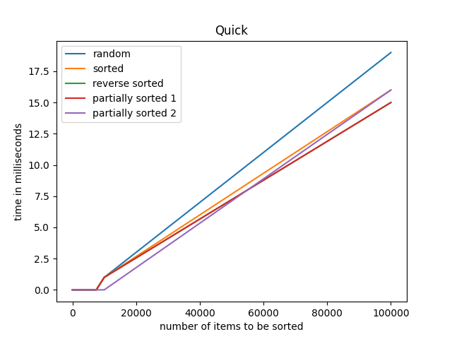
Once we have generated our arrays we can easily find out the time taken to sort the arrays and map them onto a graph. Here are some of the graphs that I have generated:
