Word Embeddings
The concept of word embeddings stems from the challenge of figuring out how to represent words when training language models.
The simplest approach to representing words in numerical format is to create a mapping of all the words in the dictionary to a unique number. So, we would first create a vocabulary like so:
{
  "a": 1,
  "apple": 2,
  "abacus": 3,
  ...
}
Then we would use it to convert a sentence like this
The trees are swaying gently in the breeze
to a sequence of indices like so
[27, 62, 10, 55, 22, 35, 27, 15]
The drawback of the previous representation is that the model might misinterpret words having similar indices to have similar meaning.
In the above example, the model might think that apple and abacus are similar even though they have no relationship with each other.
One-hot encoding
To combat this, we use the concept of one-hot encoding. One-hot encoding in a technique where we create a binary representation of each word, i.e.,
Instead of representing words with a single number like before, we represent them with a sequence of length = size of the dictionary like so:
| Word | a | apple | abacus | … |
|---|---|---|---|---|
| a | 1 | 0 | 0 | … |
| apple | 0 | 1 | 0 | … |
| abacus | 0 | 0 | 1 | … |
One-hot encoding too has a few drawbacks:
- If the size of our vocabulary is too large, the one-hot encoding also scales up which can lead to massive number of features in our language model.
- It ignores the fact that some words can be similar and can be replaced with other words that are used in similar contexts.
Word Embeddings
Word Embeddings address the drawbacks of one-hot encoding by representing each word as a vector of n dimensions. These vectors are learned from a massive database of text collected from the internet. Word embeddings capture the semantic similarity of words, i.e., words with similar meanings that are used in similar contexts have similar vectors or embeddings.
Another advantage of word embeddings is that we can train them to be as large as we want allowing them to scale with our model.
Here is an example of word embeddings visualized after reducing them down to two dimensions using t-SNE for visualization.
You can see that semantically similar words are placed together.
These word embeddings have been trained on the Wikitext-2 dataset.
You can view my implementation of the training and evaluation of word embeddings at satwik-kambham/word-embeddings.
Word2Vec
Word2Vec is a technique that uses neural networks to learn word embeddings from a large corpus of text. There are two different models defined in word2vec
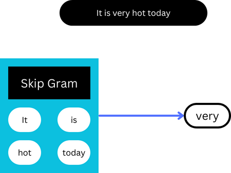
Skip-gram
Skip-gram works on the assumption that in a piece of text, a word can be used to generate its surrounding words, i.e., given a single word, the skip-gram model learns to predict its surrounding words.
Continuous bag of words (CBOW)
The continuous bag of words model works based on the opposite assumption of the skip-gram model and learns to predict the centre word in a piece of text given the surrounding words.
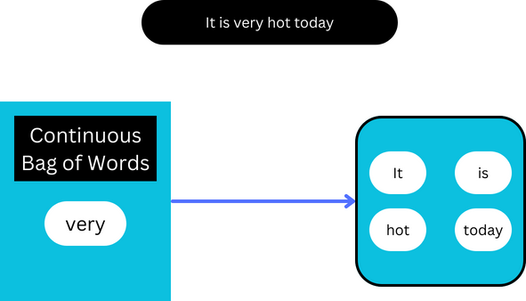
The surrounding words are also referred to as the context words.
Skip gram is better at capturing infrequent words but is slower to train while CBOW is faster to train on large datasets.
A context/window size of 10 works well for skip gram and a window size of 5 works well for CBOW.
Efficient training techniques
We can simply use cross entropy loss to train these models however for large vocabularies, it becomes impossible to use regular softmax for such a large number of categories. To combat this the following training techniques are implemented.
Negative sampling
Since, softmax is too computationally expensive to compute, one approach is to model our problem as a regression task rather than a classifier than predicts a word from the dictionary.
More specifically, we pass our model the centre word and the corresponding context words individually and it tries to predict the probability of them occurring together.
But since all the samples/pairs are occurring together, our model will not learn, so we also sample random words from the dataset and give the model negative samples so that it can learn to differentiate between words that occur together and words that don’t.
The random words are sampled from the vocabulary. The probability of a word being sampled is equal to its relative frequency in the corpus to the power of 0.75.
Hierarchical softmax
Hierarchical softmax gives us an approximation of the full softmax function using a computationally efficient approach by building a binary tree.
Hierarchical softmax is slower but works well on smaller datasets while negative sampling is very fast making it the optimal choice for large datasets.
Hierarchical softmax is better for infrequent words while negative sampling is better for frequent words and works well when producing small vectors.
Subsampling
Since, frequent words like “the”, “a”, etc. are not very useful when generating context words, our model can benefit from pruning them. So, we discard every word in our dataset with the probability sqrt(k * corpus length / count(word)). This makes it so that words that occur more have a higher probability of being removed.
Here, k is a hyper-parameter that is usually set in the range of 1e-3 to 1e-5.
We are not removing the word from the vocabulary rather we are removing a single occurrence of the word in our dataset based on the probability.
GloVe
GloVe takes a different approach to word2vec and excels at capturing long range relationships between words. It is not based on neural networks and is computationally more expensive to calculate than word2vec embeddings.
Use Cases
Word Similarity and Analogies
We can compute the similarity of two word embeddings using the following metrics:
- Cosine similarity
- Euclidean distance
- Dot product
Here is an implementation of each of the following metrics:
def cosine_similarity(embed_a, embed_b):
    return np.dot(embed_a, embed_b) / (
        np.linalg.norm(embed_a) * np.linalg.norm(embed_b)
    )

def euclidean_distance(embed_a, embed_b):
    return np.sqrt(np.sum((embed_a - embed_b) ** 2))

def dot_product(embed_a, embed_b):
    return np.dot(embed_a, embed_b)

words = ("tv", "comedy")
embeddings = [get_embedding(word) for word in words]
cosine_similarity(*embeddings), euclidean_distance(*embeddings), dot_product(*embeddings)

>>> (0.40642762, 4.504717, 6.872764)
We can use this to find semantically similar words given a single word:
def similar_words(word, metric=cosine_similarity):
    embeddings = get_embedding(word)
    similarities = [
        metric(embeddings, get_embedding(word)) for word in vocab.word2idx
    ]

    # Sort and get top 10 most similar words and their cosine similarity
    sorted_similarities = sorted(
        zip(similarities, vocab.word2idx), reverse=True
    )
    return sorted_similarities[:10]

similar_words("artillery")

>>> [(1.0, 'artillery'),
 (0.55945635, 'battery'),
 (0.5228575, 'battalion'),
 (0.50890076, 'regiments'),
 (0.5006646, 'shelling'),
 (0.49702987, 'ottoman'),
 (0.4927736, 'howitzers'),
 (0.4827104, 'bayonet'),
 (0.48132917, 'infantry'),
 (0.4784448, 'redoubts')]
We can also find analogies:
def analogy(word_a, word_b, word_c, metric=cosine_similarity):
    embedding_a = get_embedding(word_a)
    embedding_b = get_embedding(word_b)
    embedding_c = get_embedding(word_c)
    embedding_d = embedding_c + embedding_b - embedding_a

    similarities = [
        metric(embedding_d, get_embedding(word))
        for word in vocab.word2idx
    ]
    sorted_similarities = sorted(
        zip(similarities, vocab.word2idx), reverse=True
    )
    return sorted_similarities[:10]

analogy("son", "father", "daughter")

>>> [(0.75376076, 'daughter'),
 (0.5701034, 'father'),
 (0.4244268, 'mother'),
 (0.3807127, 'daughters'),
 (0.33759993, 'parents'),
 (0.33531103, 'eldest'),
 (0.32939386, 'susanna'),
 (0.32528082, 'married'),
 (0.32503176, 'meri'),
 (0.31788656, '1616')]
With language models
We can also use word embeddings in conjunction with large language models for various tasks like machine translation, text generation, summarization, etc.
Conclusion
Word embeddings are a great way of representing text and helps the model identify semantically similar words. However, pre-trained embeddings like word2vec has a few downsides:
- It cannot handle out of vocabulary words. For example, if our vocabulary has the word
toothbut not the wordtoothless, our model fails even if it has seen other relationships like this before. - Word embeddings also completely ignore spaces which can be a major downside when working with language models which are based on understanding code.